Cambridge IGCSE Physics · 0625 · Paper 6
Paper 6 Skills: Alternative to Practical
AO3 · Experimental skills and investigations
What Paper 6 tests
Paper 6 (Alternative to Practical) is a written exam of practical skills. Typical tasks include:
- Reading instruments and recording results in tables.
- Plotting graphs, drawing a best-fit line, and finding a gradient.
- Identifying variables and writing a clear method.
- Drawing or completing circuit diagrams and ray/pin diagrams.
- Suggesting sources of error and improvements.
Measurement techniques are introduced in Chapter 1. Circuit symbols: Chapter 4.3.
Variables & fair tests
- Independent variable (IV)
- The factor you change (e.g. length of pendulum, load on a spring).
- Dependent variable (DV)
- The factor you measure (e.g. period T, extension).
- Control variables
- Everything else kept constant (e.g. same bob mass, same spring, same room temperature).
| Investigation | IV | DV | Controls (examples) |
|---|---|---|---|
| Pendulum | Length l / m | Period T / s | Same bob; small angle; same timing method |
| Spring | Load / N | Extension / mm | Same spring; same zero reading; vertical set-up |
| Wire resistance | Length / m | Resistance / Ω (or V and I) | Same wire thickness; same temperature |
Measuring length, time & reading scales
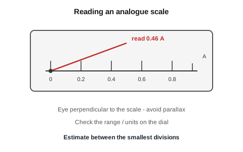
- Length: metre rule; eye perpendicular to the scale to avoid parallax.
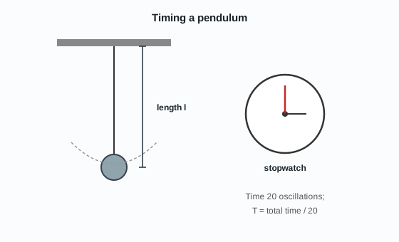
- Short times / pendulum: time many oscillations, then divide. T = total time ÷ number of oscillations. Start and stop at the same point in the swing.
- Volume: measuring cylinder — read the bottom of the meniscus at eye level.
On analogue meters, read to the nearest half-division (or better) and check the range and unit on the dial.
Circuits for Paper 6
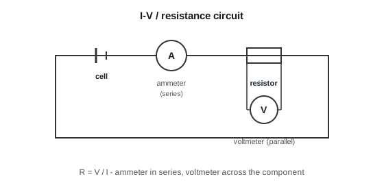
For current and potential difference investigations:
- Place the ammeter in series with the component.
- Place the voltmeter in parallel across the component.
- Resistance R = V / I (when asked).
Results tables
Column headings need quantity and unit. Include repeats and a mean when you take more than one reading.
| Load / N | Length 1 / mm | Length 2 / mm | Mean length / mm | Extension / mm |
|---|---|---|---|---|
| 0.0 | 150 | 150 | 150 | 0 |
| 1.0 | 162 | 163 | 162.5 | 12.5 |
| 2.0 | 175 | 174 | 174.5 | 24.5 |
| 3.0 | 187 | 188 | 187.5 | 37.5 |
| 4.0 | 200 | 199 | 199.5 | 49.5 |
Extension = mean length − original (unloaded) length. Check for a zero error on the metre rule or newton meter before you start.
Graphs & gradient
- IV on the x-axis, DV on the y-axis; label with units.
- Use an even scale that fills the grid.
- Draw a best-fit straight line or smooth curve — not join-the-dots.
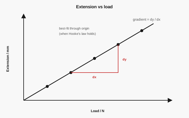
- For a straight line through the origin (e.g. Hooke’s law), gradient = Δy / Δx from a large triangle on the line.
Use as much of the line as possible. If extension increases by 37 mm when load increases by 3.0 N, gradient ≈ 37 ÷ 3.0 = 12 mm/N. That gradient is related to how stretchy the spring is (larger gradient = more extension per newton).
Exam Traps
- A tiny gradient triangle on only two close points loses accuracy marks.
- Forcing the line through the origin when the data clearly miss it (zero error) loses marks.
Density by displacement
For an irregular solid: measure mass on a balance, then find volume from the rise in water level in a measuring cylinder. Density = mass ÷ volume. Full method: Chapter 1.4.
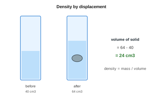
Worked numbers: mass = 72 g, volume = 24 cm3. Density = 72 ÷ 24 = 3.0 g/cm3. Keep units consistent (g and cm3, or kg and m3).
Optics on Paper 6
Ray and pin experiments (reflection, refraction, lenses) usually ask you to:
- Draw incident, reflected or refracted rays as straight lines with arrows.
- Mark the normal as a dashed line at 90° to the surface.
- Use two pins on the incident ray and two on the emerging ray so the line of sight is definite.
- Measure angles with a protractor; keep your eye above the mark to avoid parallax.
Lens and refraction theory: Chapter 3.2.2 and Chapter 3.2.3.
Cooling curves
Record temperature against time as a liquid cools and solidifies. A pure substance shows a horizontal plateau at the melting / freezing point while the state is changing. A mixture often freezes over a range (no sharp plateau).
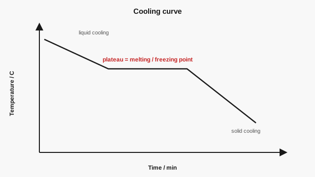
| Time / min | Temperature / °C |
|---|---|
| 0 | 85 |
| 2 | 72 |
| 4 | 61 |
| 6 | 61 |
| 8 | 61 |
| 10 | 52 |
From 4 to 8 min the temperature stays at 61°C — that is the melting point of this sample.
Errors, accuracy & improvements
- Accuracy
- Closeness to the true value — careful reading, calibrated instruments, reduced parallax.
- Precision / reliability
- Repeats close together — more repeats; better timing technique.
- Zero error
- Instrument does not read zero when it should — note the offset and subtract it, or zero the instrument.
- Human reaction time on a stopwatch → time many oscillations / use light gates.
- Parallax on a rule or meter → eye in line with the mark.
- Spring / wire heating → switch off between readings; allow cooling.
- Only a few values of IV → use at least five evenly spaced values.
| Experiment | Named precaution |
|---|---|
| Pendulum | Small amplitude; time many swings from the centre |
| Spring / load | Wait for the mass to be still; avoid exceeding the elastic limit |
| Resistance wire | Low current or switch off between readings so the wire does not heat |
| Density | No air bubbles on the object; read the bottom of the meniscus |
Writing a method
- Aim — one sentence.
- Variables — IV, DV, controls with quantities.
- Apparatus — list with ranges/sizes where useful.
- Method — numbered imperative steps.
- Safety — e.g. hanging masses securely; electrical hazards; hot objects.
- Table and graph — headings with units; state axes.
Full worked example — pendulum length and period
Plan an investigation to find how the length of a simple pendulum affects its period.
- Independent variable
- Length of pendulum l (e.g. 0.40 m, 0.50 m, 0.60 m, 0.70 m, 0.80 m) measured to the centre of the bob.
- Dependent variable
- Period T / s (time for 20 oscillations ÷ 20).
- Control variables
- Same bob; small amplitude each time; same timing point in the swing; same support.
- Outline method
-
- Set the pendulum length to 0.40 m using a metre rule.
- Displace the bob by a small angle and release.
- Start the stopwatch as the bob passes the centre; time 20 complete oscillations.
- Calculate T = total time / 20. Repeat twice more; find the mean T.
- Repeat for the other four lengths.
- Plot mean T (y) against l (x), or T2 against l if asked to linearise.
Second worked example — resistance and length of wire
Plan an investigation to find how the length of a resistance wire affects its resistance.
- Independent variable
- Length of wire (e.g. 20 cm, 40 cm, 60 cm, 80 cm, 100 cm) measured with a metre rule.
- Dependent variable
- Resistance R / Ω, found from V and I (R = V / I).
- Control variables
- Same wire (same material and diameter); same ammeter and voltmeter; keep current small so temperature stays roughly constant.
- Outline method
-
- Connect a cell, switch, ammeter, and the wire in series; connect a voltmeter across the chosen length.
- Set the contacts 20 cm apart. Close the switch, record V and I quickly, then open the switch.
- Calculate R = V / I. Repeat twice more at this length; find a mean R.
- Repeat for the other four lengths.
- Plot mean R (y) against length (x). Expect a straight line through the origin if temperature is constant.
Gradient example: If R increases by 4.0 Ω when length increases by 0.80 m, gradient = 4.0 ÷ 0.80 = 5.0 Ω/m — resistance per unit length of that wire.